
Screen Shot 2026-03-02 at 4.18.40 PM.png
- 444.29 KB
(2003x1640)


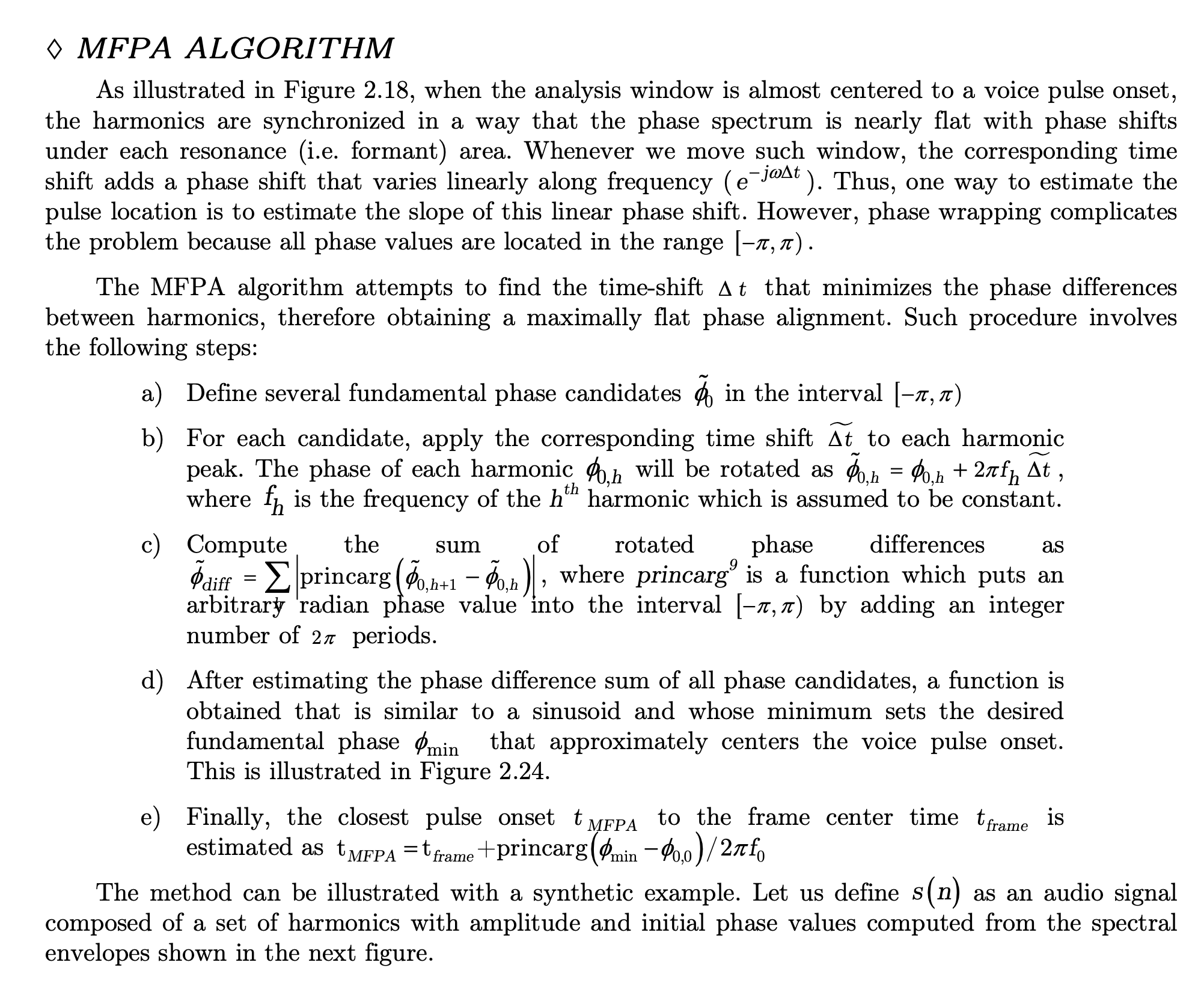
So I've been working on a project to create a singing voice synthesizer I'm basing it on the description in Jordi Bonada's PhD thesis "Voice Processing and Synthesis by Performance Sampling and Spectral Models". After a lot of trouble with getting TWM f0 estimation to work, I've finally gotten to implementing MFPA (Maximally Flat Phase Alignment". And amazingly, it seems to have worked first try. Compare my results: https://i.ibb.co/dsvgv0fd/Screen-Shot-2026-03-02-at-3-54-48-PM.png To the results in the study: https://i.ibb.co/C3fjdWVd/Screen-Shot-2026-03-02-at-3-55-09-PM.png
Screen Shot 2026-03-30 at 4.51.32 AM.png
- 92.20 KB
(1132x839)

Hello, I'm back and I have a major update to my VOCALOID project! I have sucessfully achieved a shape-invariant pitch transposition! Here it is. First the original audio: https://files.catbox.moe/zmt3rr.wav Now my version with WBVPM (pitched down by an octave): https://voca.ro/1mJ5qljrp9hD or https://files.catbox.moe/kho97n.wav And a version using a naive pitch shift: https://files.catbox.moe/xs39bq.wav Notice that my version, while having more noise, sounds more natural and has less phasiness. This is particular noticeable if you play both at very low volume. One sounds much more 'human' than the other. Also note that this an extreme example with an octave shift (or 1200 cents) - in practice, shifts would typically be far less. Also this doesn't implement several other parts of the system (more on that later). I'll explain all of this in a moment, but first, I'd to correct some major biographical errors. Since this is a long post, I've divided it into sections BIOGRAPHICAL CORRECTIONS In the last post, I claimed that VOCALOID1 used Narrow-Band Voice Pulse Modeling while VOCALOID2 and onwards used Wide-Band Voice Pulse Modeling. This was incorrect, and additionally it was the source of most of my confusion surround the paper. What actually happened is that the research technology that would later become VOCALOID1 started out as work to improve the existing Spectral Modeling Synthesis system that had been developed in the early 1990s. This improvement began work in the late 1990s. But importantly, this system evolved and techniques from it were incorporated with techniques from a system that was being developed called a Phase-Locked Vocoder, and this system would be released as VOCALOID1. In the mid-2000s, work began on combining the techniques learned from improving SMS and the PLVC-based system and attempting to combine them with the mucher older and well-known TD-PSOLA system. Importantly, TD-PSOLA (Time-Domain Pitch Synchronous OverLap and Add) was a time-domain system, while SMS was a frequency-domain system (and also TD-PSOLA was pitch synchronous - hence the name, while SMS had a constant hop size). The first technique they developed was Narrow-Band Voice Pulse Modeling, and later Wide-Band Voice Pulse Modeling. Wide-Band Voice Pulse Modeling ended it up being used in VOCALOID2. Now that I understand this, I also understand the major mistake I made when reading the paper: I was reading it from the perspective of an implementer, thinking of the sections as the steps to implementing it instead of as research. I had thought that section 2.2 described the core processing algorithms. When it was actually about SMS, and importantly, about *the improvements they made to SMS*, and not a complete description of SMS, since SMS was already an established technique. Hence my confusion on why some things were seemingly vaguely explained, since *the paper wasn't about them*. At the same time, much of that section is very useful though because importantly, much of that research was also incorporated into the later techniques. RESULTS I have successfully implemented the Wide-Band Voice Pulse Modeling; synthesis; and pitch transposition, time stretching, and timbre scaling algorithms. Additionally, I have also finished implementing the full version of the pitch estimation module, changed the code to work using overlapping windows, implemented the window adaption system, and fixed countless.
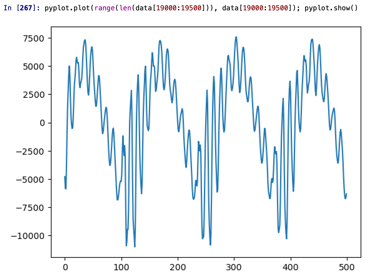
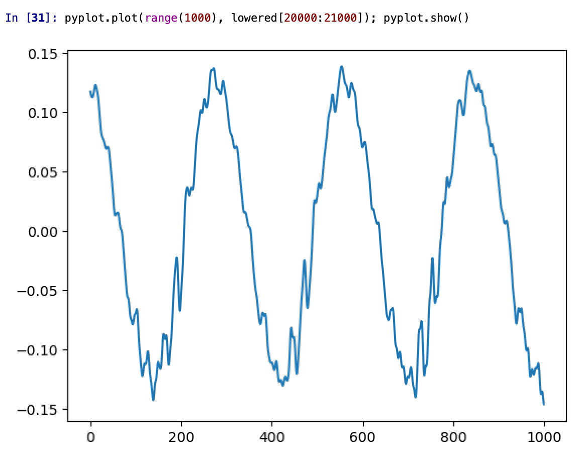
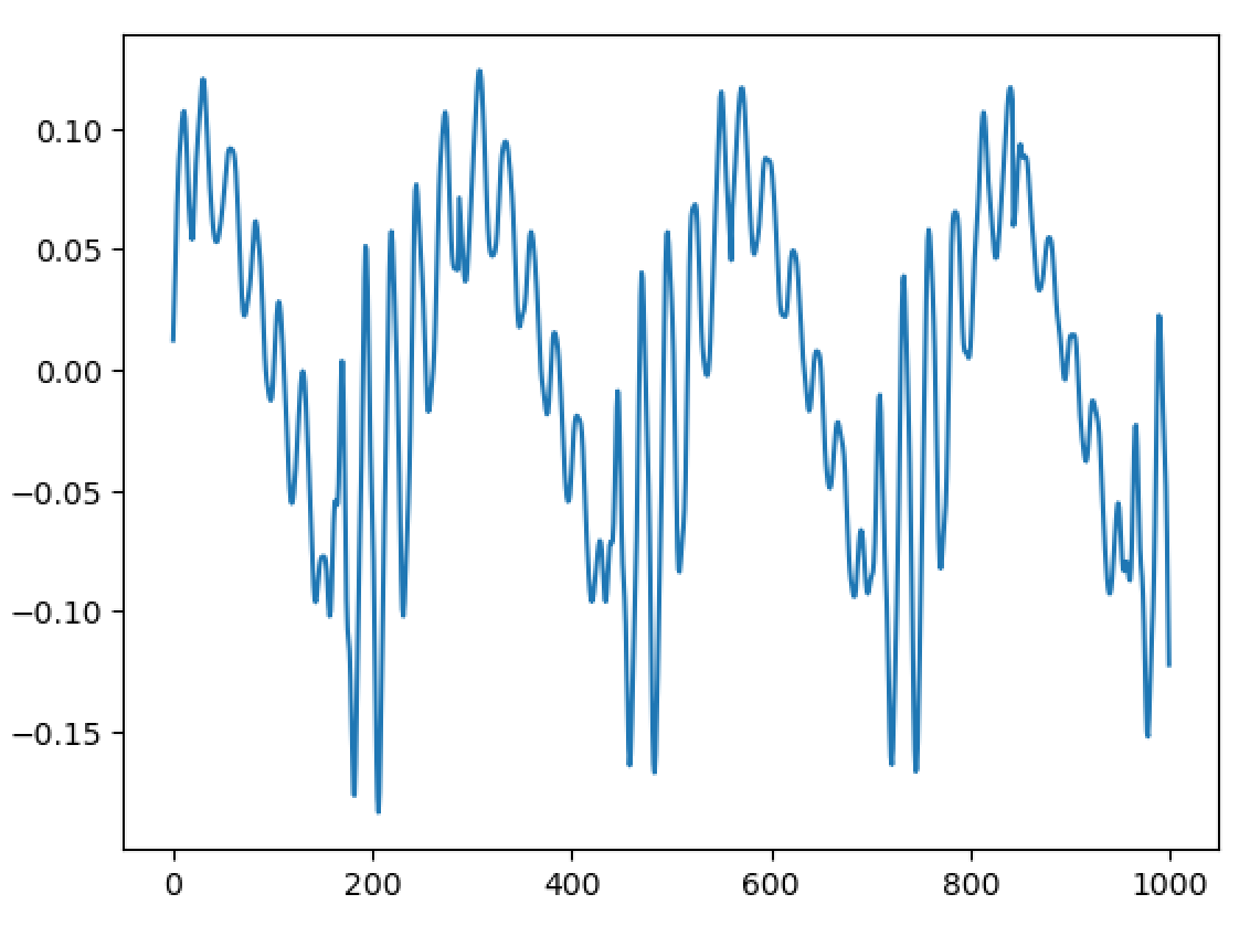
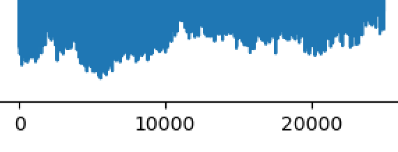
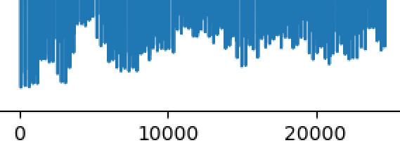
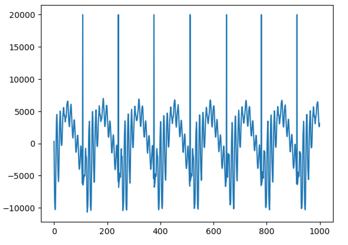
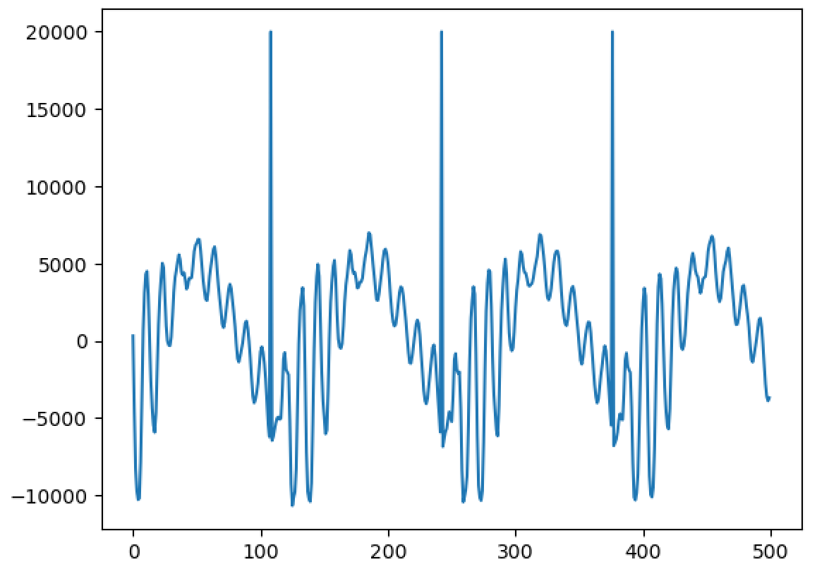
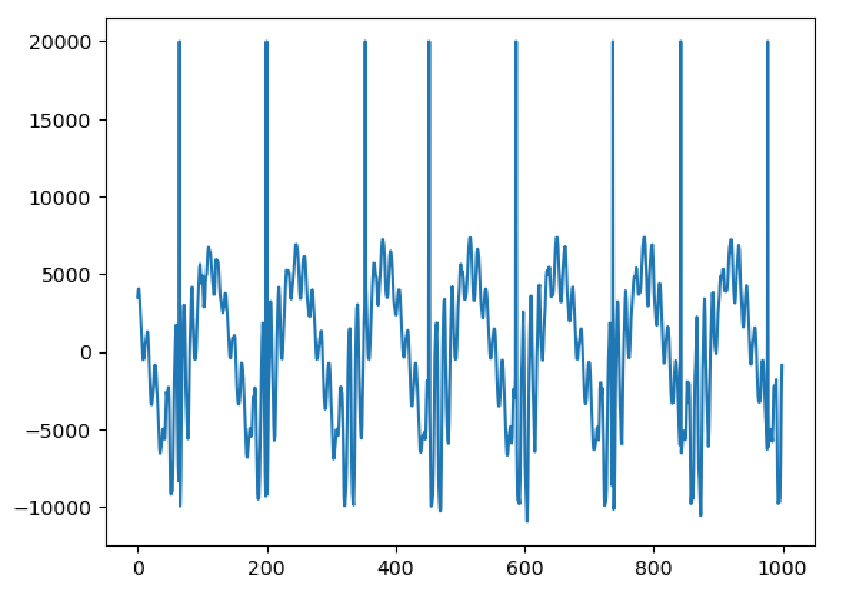
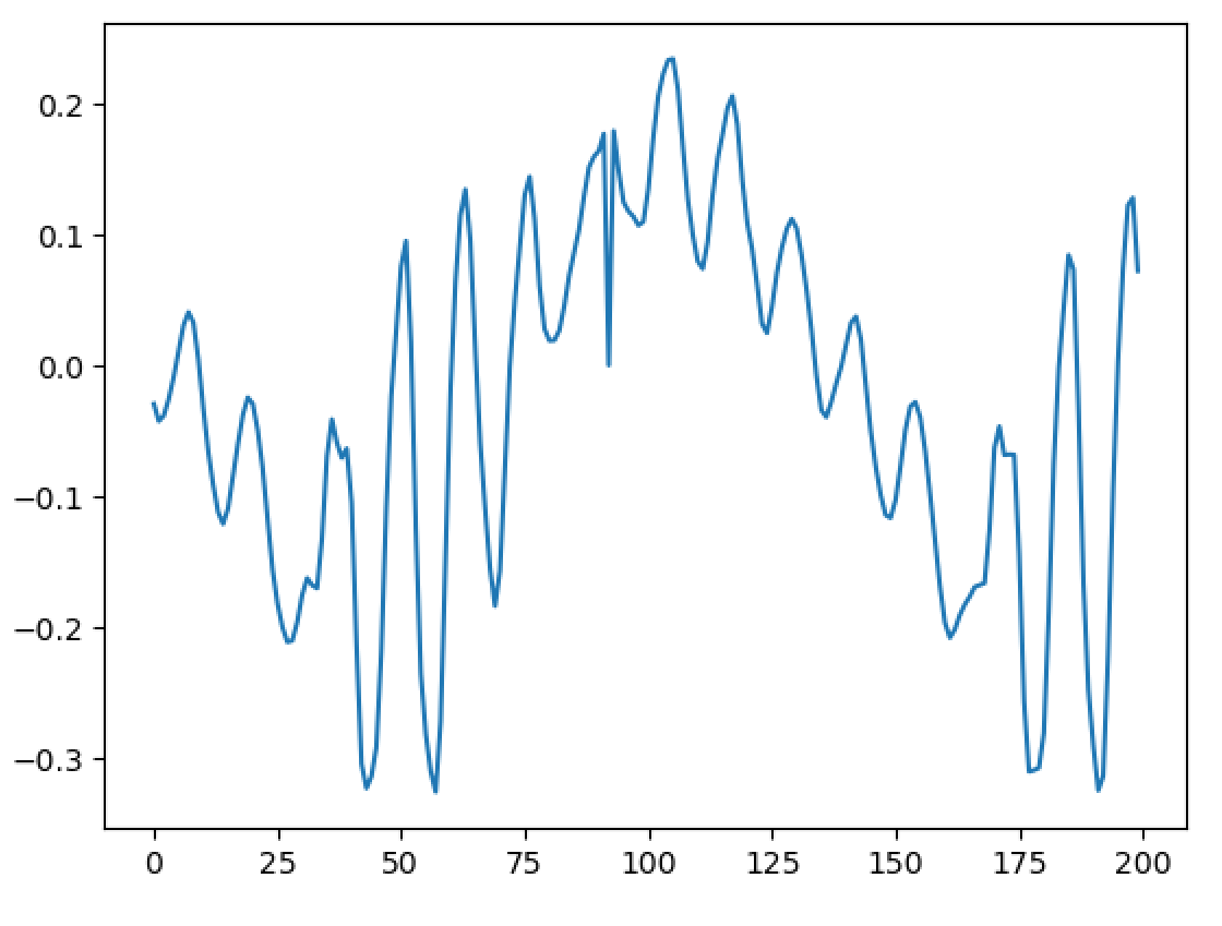
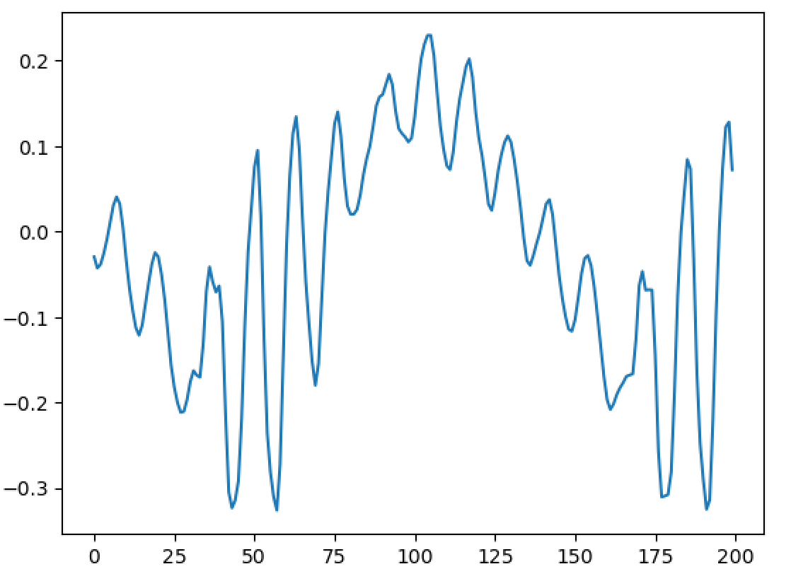
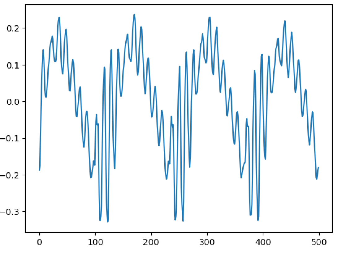
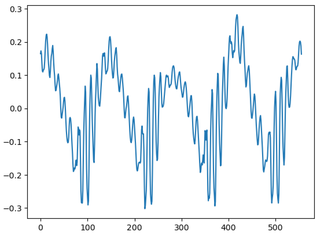
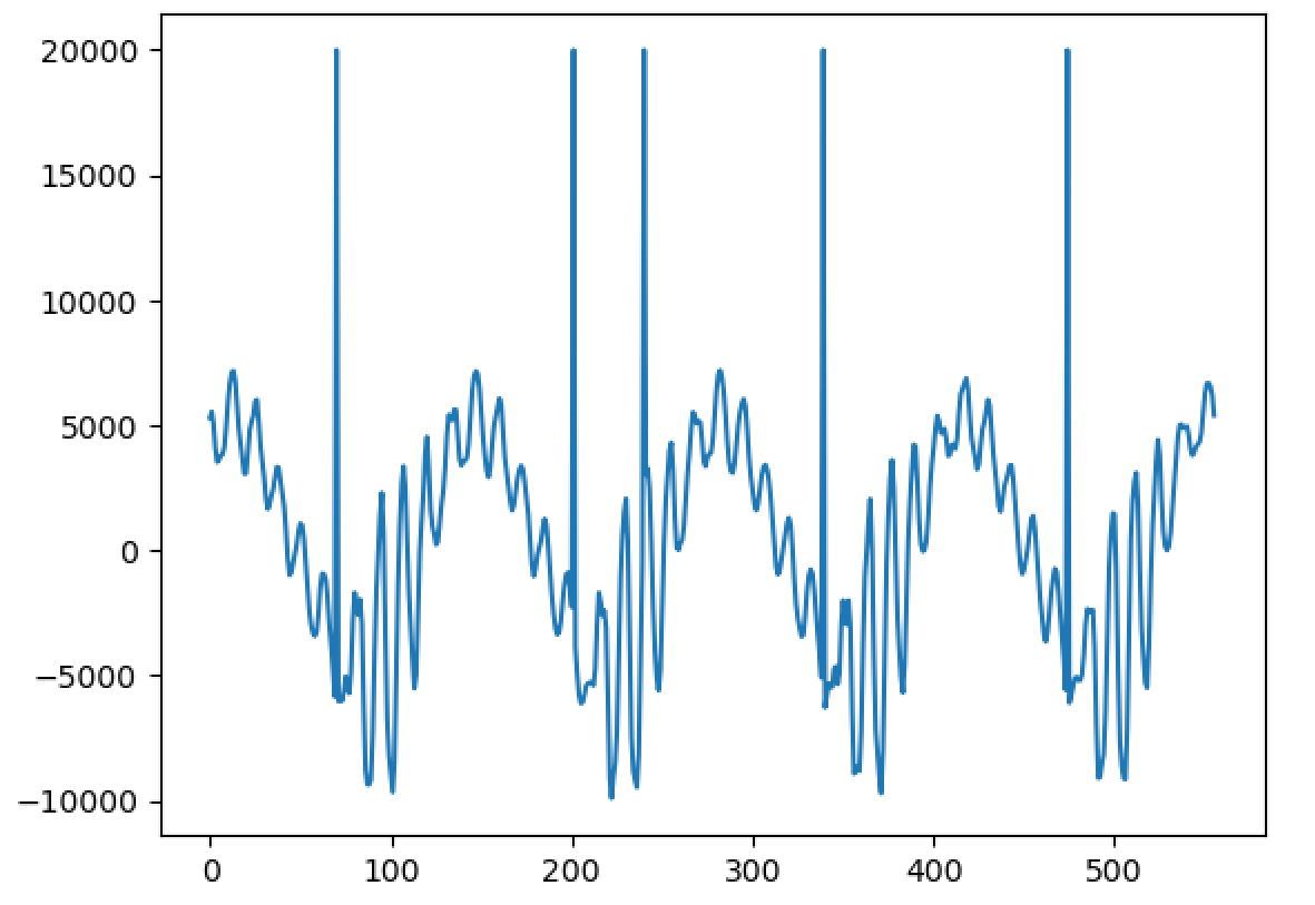
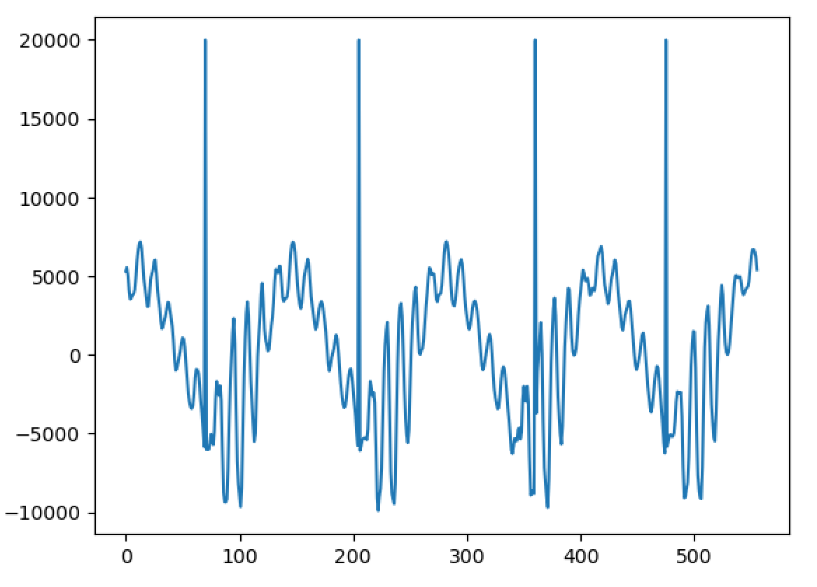
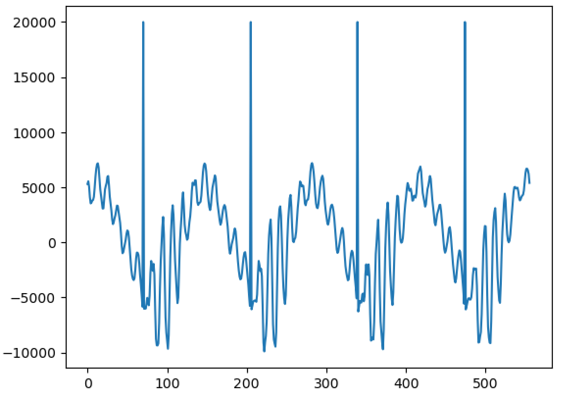
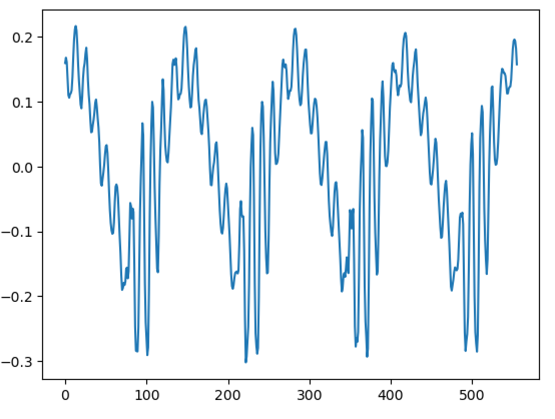
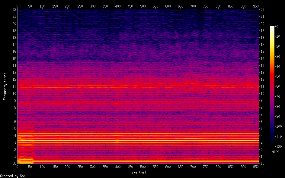
Importantly, I have been able to experimentally replicate a very important property - and one of the main reasons WBVPM was developed, in fact. That property is shape-invariance. You see, an important property of the human voice is that, all else being equal, the shape of each pulse in the waveform stays roughly the same regardless of frequency. The reason for this property is phase-coherence. At the start of each voice pulse (when the glottis closes), the phases of all the harmonics within each formant (where each 'formant' is a spectral region affected by the vocal tract differently) are roughly the same. Since phase changes proportionally to frequency, the different harmonics will shift from that point over time, and soon become very different from one another. Since the phases are vastly different with relation to the frequency at times other than the voice pulse onset, the harmonics interfere constructively and destructively in the time-domain. Importantly however, if all the harmonics are scaled equally, the phases all now change at a slower or faster rate, but importantly this rate scales the same for all of them. This gives rise to shape-invariance, since the pattern of interference stays the same, just at different scales. Importantly, if you apply a transform relative to a point that is not a voice pulse onset, the phases will not be flat. Of course, that transform can shift the changes *from* the point it started from, but importantly it is NOT accounting for inherent phase shift that occurs from not being at a voice pulse onset. Of course, if no transform is occurred, then there will be no issue. But if one is, say a pitch transposition, then the initial phases from the starts if signal was actually shifted to the pitch originally will differ considerably from the observed ones since the observed ones base themselves on the measured phase *at a different pitch*. This results in the breaking of shape-invariance, a noticeable 'phasiness' sound, and the sound sounding un-human. Here is an image of 500 samples from the original signal: https://files.catbox.moe/223l7p.png Now here is 1000 from a one octave down pitch transposition using a naive approach (a fixed-window and hop-size approach using a 1024-point Hann window): https://files.catbox.moe/jxgtg0.png Notice that not only is the waveform unrecognizable compared to the original, it even varies considerably between individual voice pulses! Now compare to 1000 samples from the WBVPM approach: https://files.catbox.moe/6hpf8l.png Notice how the waveform is almost identical, only scaled up two times in period, and it varies much less. You may be wondering, couldn't we just downsample or upsample the signal and play it back at the same sample rate to get the same result? Well, importantly, we have independent control over pitch and time. In the example, I downsampled the voice by a factor two, but kept the time the same and it contains the same number of samples as the original. Additionally, in the analysis and then synthesis reconstruction, it is seperating it into individual voice pulses. Importantly, it isn't just scaling them, it is generating new voice pulses in the frequency domain and inserting them at positions that were also generated. Here is an amplitude envelope of the latter half of the original audio: https://files.catbox.moe/6zw5v5.png Now here is an amplitude envelope of the latter half of the pitch-transposed audio: https://files.catbox.moe/2a3utu.png Notice how they a roughly the same. If the audio was just downsampled, the second would be stretched out by a factor of two - but is not. I also implemented timbre-scaling, although I have not tested it. Fun fact; when I implemented it, actually did so by accident. I was trying to implement the pitch transposition, got a bit confused, and realized I had also accidently implemented timbre scaling.
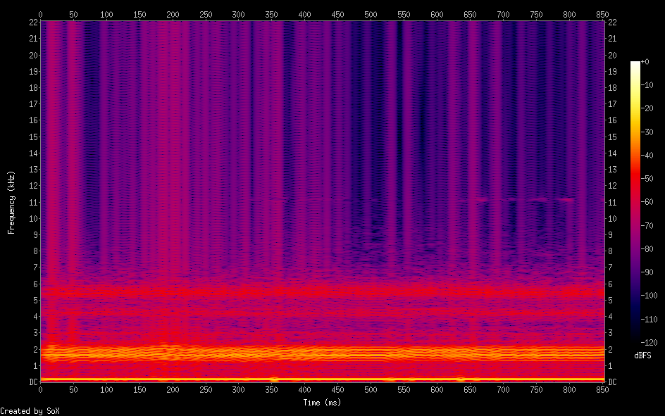
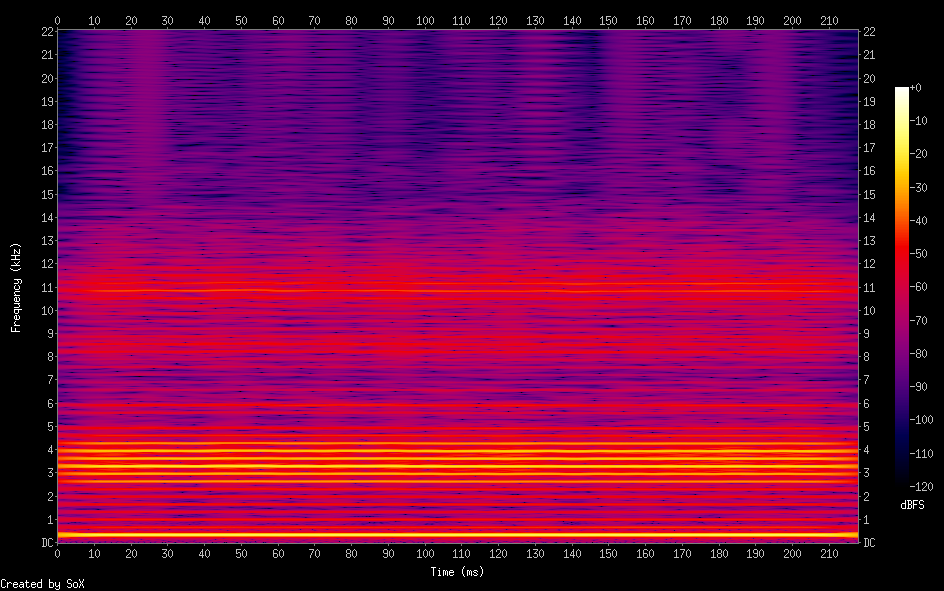
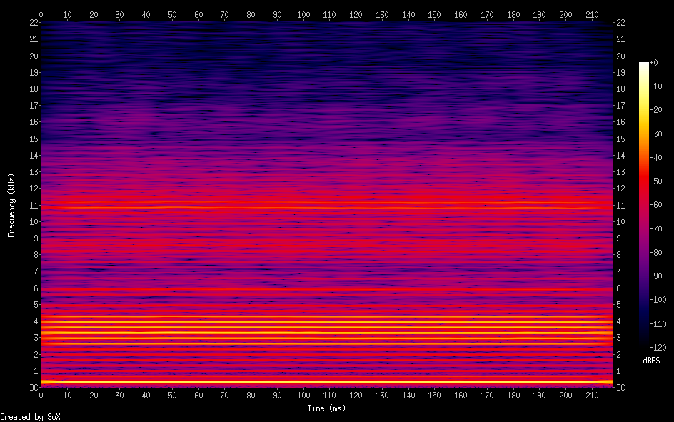
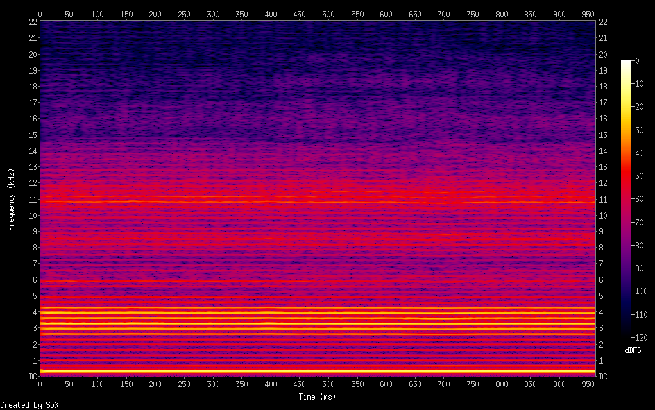
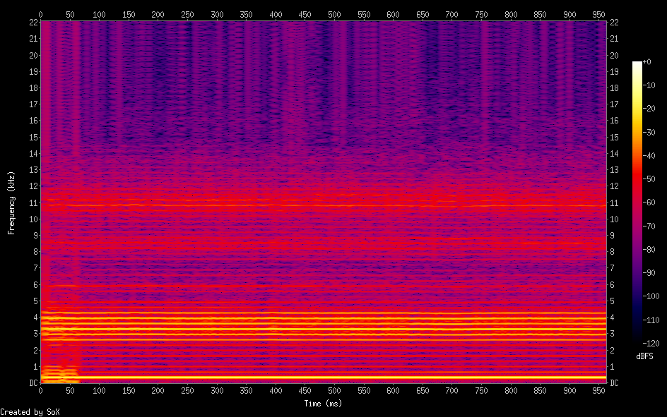
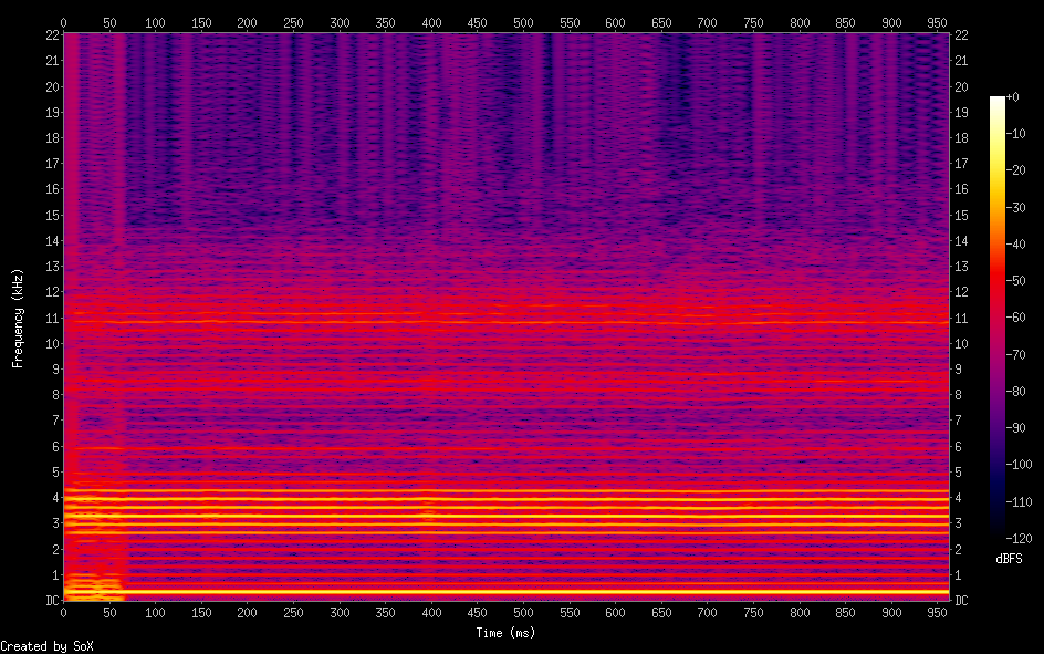
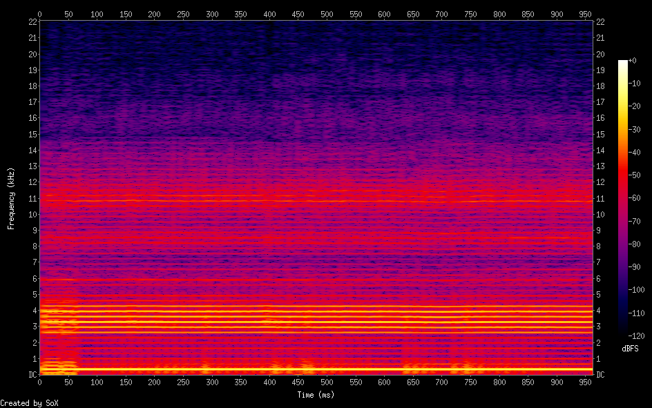
All these transforms are currently implemented as linear transformers. However, they are all implemented by just sampling a spline at a regular interval, so they could be trivially made to accept a non-linear parameter, sequence of points, or spline instead. Although this current implementation is far from perfect, I think it works reasonably well as a demonstration of the techniques and their properties. Keep in my mind that I have done nearly no adjustment of the constant parameters/'tuning'. In fact, there are several parameters whose corresponding feature is effectively disabled because I wasn't sure what value to pick. This implementation could probably be considerably improved just by adjusting a few constant. An (hopefully) efficient and accurate way of 'tuning' automatically is discussed later in this post. Notably, the pitch-transposed spectrum varies significantly, with some areas showing little residual and straight lines: https://files.catbox.moe/04naz0.png (those lines in some areas around the center of the spectrum are probably the aliasing artifacts Bonada 2008 mentioned in WBVPM when using upscaling, I will implement the method for avoiding them at some point) Additionally, I have also tested reconstructing the sound with no transforms. This seems yield little residual, although it seems concentrated at higher frequencies, so maybe that can be fixed. Maybe it could also be caused by aliasing. Here is an audio file that was reconstructed through the WBVPM synthesis procedure using downsampling: https://files.catbox.moe/bhxjpw.wav And a spectrogram: https://files.catbox.moe/kvrnkq.png Compare to the spectrogram of the original: https://files.catbox.moe/d1vo16.png PITCH ESTIMATION Throughout this project, the most finicky part has been - and continues to be - the pitch estimation; specifically the Two-Way Mismatch algorithm for monophonic pitch detection. I have compiled several variations of the TWM algorithm. I tested one change that worked by scaling a term by the amplitude (I had actually though of this idea myself, and this term happened to be the term I mentioned causing me trouble last time), and it led to considerable improvement so I kept it. There's also the adaptive window procedure that wraps the TWM f0 estimation. One thing I had been noticing for a long time was that Kaiser-Bessel beta values about 10% higher than the recommended values given in Cano 1998 seemed to perform much better. I had assumed this was just because of issues with my code, or the audio samples I was testing on. Much later, I was experimenting in python when I noticed a function called kaiser_beta which converted something else abbreviated to 'a' to the equivalent beta value. Previously in Cano 1998 and in other places, I had seen the Kaiser-Bessel parameter as alpha instead of beta. Up until this point, I had either not paid attention to this, or I had assumed that these had referred to the same thing. I did some research and found out that it converts between attenuation and the beta value for the Kaiser-Bessel window. Then I found that there is indeed an alpha form of the parameter and it is not that same as beta. Confusingly however, it is not attenuation, but both abbreviate to the same thing. The Kaiser-Bessel beta can be determined by just multiplying the alpha value by pi. Interestingly, this is much higher than the 10% I tested, however it seemed to perform better (or at least not worse) anyway. A possible explanation for this discrepancy is that the adaptive window is larger than the window I used to test the adjustment originally.
Another improvement relating to windows is the window used for the harmonics that are fed into MFPA. Originally, I had used the same Kaiser-Bessel window for both. I later switched to a Blackman-Harris -92dB window, which I had seen mentioned in the paper. This resulted in a significant improvement. Another improvement I tried was adapting the window size to a value relative to the period of the estimated fundamental frequency. I tried doing this - using the same number of periods as are used for the Kaiser-Bessel window used for TWM - and noted a substantial improvement, even more so than the improvement from switching to the Blackman-Harris window in the first place. Indeed, this matches the results contained in the study. In the WBVPM section, they observe a considerable improvement (up to -10dB) when using an adaptive window size when compared to a fixed window for narrow-band analysis. In that same section, they also found 2 to be the ideal number of periods for minimizing noise and also did experiments with a Hann window. Perhaps experimenting with these ideas could lead to improvements, although that section is about getting an accurate spectrum and reconstruction, which may differ somewhat in needs from the needs of MFPA. Another idea could be using a separate function for determining its adaptive number of periods, as opposed to using the same value as for the Kaiser-Bessel window as I am currently doing. Perhaps always using an integer number of periods could be beneficial. Another idea is only using one or two periods, which would provide better time resolution, and could be better suited for wide-band analysis as we are doing. Another potential improvement I have thought of, but not yet tested, is modifying the constant parameters of the Blackman-Harris window in a manner similar to the method Cano 1998 describes for the Kaiser-Bessel window beta (and that I have used for that), where the constant parameters (or in this case, parameters) are modified in accordance with the fundamental frequency. Another potential for improvement of the MFPA results could be the use of a peak selection algorithm. I had previously used a very simple one I had found on another resource by the UPF Music Technology Group. Although this algorithm did not seem to show an improvement. I later removed it and saw no observable detriment. The paper does not provide details on this specifically, but I now understand why, so I should do more research with how this was tackled in SMS. One idea I've though of myself is to calculate the estimated harmonics and then search the surrounding area for peaks. We then select the peak with the minimum error, where that error is determined based on distance and amplitude. One formula I have thought for the error calculation but not tested is amplitude / distance^2. We want to search far enough to always have the best candidate, but not too far is to be computationally inefficient or run into floating-point error and instability in the error function. A potential improvement to this approach is instead of determining the initial estimate for the harmonic frequency by multiplying the fundamental frequency by the harmonic index, we could instead add the fundamental frequency to the peak that was chosen to be the last harmonic. This would account for drift caused by inaccuracies in the f0 estimation and also distortion in the harmonics. However, this also runs the risk of drifting away from the harmonics. A possible solution to this issue could be blending this estimated harmonic frequency with the one obtained by multiplication with the fundamental frequency. This could act as a sort of course correct that would work gradually, but at the same time keep the benefits of basing it on the previous selected harmonic peak.
Another potential improvement could be found by fixing sudden jumps in fundamental frequency that last for only a few analysis frames and then return to roughly the same fundamental frequency as before the jump. Cano 1998 calls for a "hystheresis cycle" - though I am not sure exactly what that means. I have implemented a simple system that discarded large relative jumps that last for only a single frames. However, this has two major issues. The first is that these jumps often last for more than just one frame. The second is that if I legitimate jump in f0 that stays occurs, this introduces one frame of lag. MAXIMALLY FLAT PHASE ALIGNMENT My last post was about MFPA, since then, I have made a number of improvements to this part of the system. I don't believe I have made any changes to the core MFPA function itself, but I have made a lot of improvements to the MFPA refinement algorithm as well as the code surrounding MFPA. One major improvement I made only recently. The previous issue stemmed from what I now believe to have been a misunderstanding. The MFPA algorithm gives a phase shift for each frame. This can be converted into a time offset. However, unless the frame-rate is exactly the same as the fundamental frequency (in the instantaneous sense), this will give more or fewer pulse onsets than actually exist. At the time, I was using a high-pitched sample for testing whose f0 was much faster than the analysis hop-size of 256 samples (or ~172 per second at 44.1kHz). Because of this, there were usually more than one pulse in between each detected pulse onset. At the time, I had thought that getting all the pulse onsets was the purpose of the MFPA refinement algorithm. Which is why I was confused that the it was described as choosing a *subset* of the pulses and not a superset. At the time, I had implemented the MFPA refinement algorithm, but it was buggy and either didn't work or did nothing. Later, I began thinking of ways myself of getting the in between onsets. My ideas was to add increments of the f0 period until the next pulse was reached. I eventually realized that the purpose of MFPA refinement algorithm was not interpolation, but to take a list of pulse onsets that could include multiple close estimates for the same pulse and narrow it down so there is only per pulse and such that the best one is chosen (actually it looks at a few additional candidates, which somewhat tripped me up into thinking it was about interpolation for long). For this to happen, the analysis hop-size needs to be greater than the fundamental frequency (if it was equal, it would likely slowly drift and eventually miss one onset). I realized the issue why the hop size was high (and thus the maximum frequency low) in the paper was that they were using low frequency audio samples in the range of 50-100Hz, while I was using samples around 300Hz. I adjusted to the hop size to 96 and got great results. I think I had also tried this before, but it had not worked, and it couldn't have, because this is only possible without decreasing the size of the analysis window within the overlapping window framework, which I had not implemented yet at the time I first tried. However, this low hop size is relatively computationally expensive, so much so that f0 and MFPA peaks take up most of the execution time. A possible improvement would be to use a lower analysis rate and actually use the interpolation method, but then feed the interpolated pulses into the MFPA refinement algorithm as you would likely get better results that way. I have fixed numerous bugs within the MFPA refinement implementation. A noteworthy one is that previously, I was not considering that the analysis window's time is in the center, and not the start. Because of that, the new onsets are now offset compared to the old ones, but I believe it is now correct.
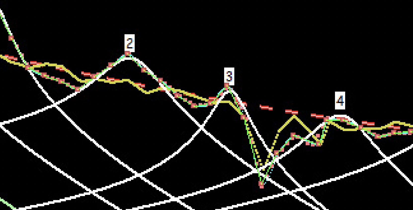
The pulse onset selection is now quite good: https://files.catbox.moe/ik27fw.png Close up: https://files.catbox.moe/urby2w.png However, there are still deviations. Here is one at around 20k samples in one of my test audio samples: https://files.catbox.moe/76nlgo.png So there is still some work to be done. Another potential improvement could be the introduction of a system for detecting for formants and weighting them less in the MFPA calculation. Recall that phase is roughly constant within a formant, but not between them. START FRAMES In the audio samples I have provided so far, I have cut off the first part of the audio. The issue is with pitch estimation for early frames. Remember that are analysis window is multiple f0 periods in size. Because of this, it can't fit at the start so it has to be decreased to a much smaller size. This is much more of an issue now that I have decreased the hop size substantially. I have now set it to skip the first few frames, because otherwise, the forced extremely small window size causes the whole pitch estimation system to irreversibly destabilize. I've been thinking of solutions to this problem. One solution could be to let the analysis window take on the full size it wants and pad the area before the start with zeros or maybe something else, this could also be used for the end. Possibly the most promising solution I have come up with, although I have not test any of these, is to back fill the previous the pulses with the first good estimated pulse onset minus integer multiples of the first good estimate of the fundamental frequency. This should work assuming both the first pulse and fundamental frequency estimate are good, the fundamental frequency stays relatively constant over the start section, and the start section only contains a few pulses. Luckly the last criteria will always be satisfied as the size of the start section is half the size of the window, and the number of pulses is then (window_size / period) / 2, but the window size in the adaptive framework is just a small number of periods, so we are left with the (mostly) constant adaptive_period_count / 2 as the number of pulses. WIDE-BAND VOICE PULSE MODELING Regarding the patent issue, I have determined that it applies only to the specific technique in Bonada 2008 WBVPM of using periodization to achieve a real-sized discrete fourier transform. However, that section also another option, that being interpolation. I have implementated it and found it to work well. I did a test a found a noise level of about -140dB (for reference, 1ulp for a single-precision float is about -145dB), which is extremely negligible and comparable to the results in the study for the periodization technique. I have also added the ability to use a few extra samples on the side to improve the spline. However, I have not tested the consequences of this variation. I don't know whether the original implementation did something like this.
Text in the patent: "generating for each pulse a sequence of repetitions of said audio pulse, said audio pulse being repeated according to its own characteristic frequency; deriving frequency domain information associated with at least some of the sequences of repetitions of said audio pulses, each said sequences of repetitions of said audio pulse being represented as a vector of sinusoids based on the derived frequency, said vector of sinusoids corresponds to a sinusoidal series expansion of the specific audio pulse;" Bonada 2008, WBVPM, NON-INTEGER SIZE FFT: "PERIODIZATION: one period of the input signal is windowed with wR (n) , and repeated several times at the rate defined by T so that the FFT buffer of length M covers in the end several periods. The repetition implies interpolating both the signal samples and the window function. Then the resulting signal sr (n) is windowed by an analysis window function wA (n) , and the spectrum obtained is actually the convolution of such analysis window response WA (f ) by the spectrum of Sr (f ) sampled at harmonic frequencies" TUNING I have come up with two techniques for tuning that apply in different ways. AUTOMATIC TUNING - The idea is that we use a stochastic statistical algorithm that minimizes a cost function by adjusting a set of parameters (one I looked into that seems promising is global-optimization SPSA). The parameters in this cases would be constant used in C. A python script would replace placeholders with the values being picked by the minimization algorithm and then compile and run the C program. The results would then be compared to a reference by another algorithm/program, which would then be summed together to give a cost value. A program for doing I plan to research is called AudioVMAF. I believe it was originally designed to test audio compression, however I hope that it could also be useful here. MANUAL TUNING - In this method, we insert instrumentation into various intermediate values calculated in the program. Then, for one very small snippet of audio, we use Automatic Tuning to determine ideal values. Then, a programmer tries to write code to make it better match these desired values. Then, if successful, it can be test in general over the whole dataset. If it is not an improvement, then the most negtaively affected audio snippets can be selected and then have a similar process to decrease the change for them while keeping the change for the ones that benefit. Both of these methods would work best for matching with another vocal synthesizer, since the timings and parameters can match exactly. However, they may also be adaptable to optimizing parameters for real-world (and thus also realistic) voices. It would have to work somewhat in reverse though in that someone would sing first and then a note sequence would have to be made that matches it almost exactly. OTHER CONSIDERATIONS There are many more potential tweaks and improvements. I have many dozens accumulated and plenty more to research, test, and implement. One widely applicable variation is using logarithmic based scales. I still don't have an answer to the voiced/unvoiced frame decision issue, but I will look for SMS research about that and older Bonada papers. One heuristic I thought of is noise / amplitude^2 > threshold.
ADDENDUM, because I just realized I forgot a bunch of things I meant to put into this post This is still a simplified model. It does not take into the Excitation plus Resonance model, the Spectral Voice Model. It uses a linear transform and not generated trajectories. One thing I was thinking about was the part in WBVPM section where they said that one of the disadvantages of WBVPM was not being able to separate harmonic and non-harmonic. I also read that the noise is embedded as fluctuations in the spectrum of each voice pulse and over time, which is what I had presumed because the information has to go somewhere. I was thinking, what if you took each harmonic as the values and the pulse onsets times as the positions in a spline. Then interpolated at regular intervals. Then applied the fourier transform. Then separate the highest frequencies and the others. Take the others and apply the inverse Fourier transform, and then rebuild a spline from this and interpolate the values back at the onsets. I wonder if this would work. There would be loss though because of the resampling steps. This could decreased by taking more samples. You could also apply a correction by sampling and sampling it back to calculate the resampling loss itself without the removal of the high frequency modulations, and then add this difference back to the main pulse information after the separation.
Hello I'm back with another update to my VOCALOID project. It's not as big an improvement as last time - and in fact, there's no new features - but I felt like it was worth posting. I've been trying to rectify the major issues before I move onto implementing the Excitation plus Resonance model. The first thing I attempted to tackle was all the added noise at high frequencies. Here's the original spectrum: https://files.catbox.moe/fq55bo.png And here's the reconstructed spectrum (with no transforms applied): https://files.catbox.moe/gq7jff.png You can clearly see the high frequency artifacts. The first thing I tried was something mentioned in the paper. In the paper, specifically the WBVPM section, it was mentioned that there are two approaches for a non-integer size discrete fourier transform. The first one is repeating the signal while second is upsampling it. I went with second as the former is patented and also because the second is easier to implement. It is mentioned that increasing the repetition count of the signal (or in the case of upsampling, the upsampling factor), and then discarding the higher frequencies, can improve the estimation by reducing artifacts. In the case of repetition, it is also mentioned that quadratic interpolation can be used in the resulting spectrum, however I am not sure if this can be done for upsampling and as such, I have not tried to implement it for now. Here's the result after applying an upsampling factor of 3: https://files.catbox.moe/qcgnzq.png Here's the original audio: https://files.catbox.moe/f7g8ta.wav The original reconstruction: https://files.catbox.moe/da0m1i.wav And now with the improved reconstruction: https://files.catbox.moe/513ycn.wav You can see an improvement, especially at lower frequency, however the high frequency artifacts largely persist. So they have to be arising elsewhere. I realized the source was the reconstruction of the signal (AKA the "synthesis"). I had previously implemented a synthesis method that was quite different from the one used in the study, because I did not understand the method in the study at first. My synthesis method worked by taking each voice pulse and for each sample where the voice pulse is the closest voice pulse to that sample, setting the value of that sample to the interpolated value of a spline representing a time domain version of the upsampled voice pulse with a step corrospondin between the ratio a sample in the regular time domain and the upsampled time domain. Now, in some cases, estimation inaccuracies and differences from any transformations that were applied result in these regions of samples being bigger than the actual sample itself. In these cases, we take advantage of the period nature of the voice pulse and repeat it (i.e. sampling before the start is equivalent from that offset from the end, and sampling after the end is the same as that offset from the start). However, this method results in discontinuities in some cases. Here is an example of such a discontinuity: https://files.catbox.moe/jnnxfj.png I began to try to implement an interpolation system. In this system, we could calculate the gap between pulses - or in the cases of inaccuracies in the other direction (i.e. overlapping pulses) - the overlapping area, and interpolate between one pulse and the other linearly. However, this was approach was complicated significantly by the non-integer (and potentially differing) sizes of the pulses as well as numerous edge cases. For this reason, I struggled to do so and spent over an hour trying to figure out how to do it corrrectly. About half way through, I decided to check the paper again and this time I understood the actual synthesis method properly, largely because of a diagram I had missed the first time.
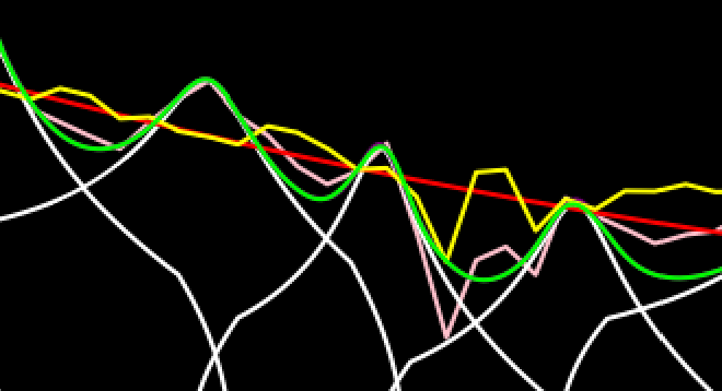
>>12281 In the actual method, each pulse is is expanded in a manner similar to that of the border interpolation technique used in WBVPM analysis, except kind of in reverse. In this technique, for each voice pulse, we generate extensions on both sides with each extension having the size of the border interpolation ratio of the size of the voice pulse. Then we apply a trapezoidal window to the voice pulse which starts at zero at each side of the extended voice pulse and becomes 1 on either side after protrusion of twice the border interpolation size on each side. Then we overlap and add the voice pulses. This technique fixes the discontinuity issue because it effectively results in each border-interpolation-length side of each voice pulse being interpolated with the corrosponding section for the other voice pulse linearly over a period of twice the border interpolation size. However, this only holds perfectly when the fundamental frequency is the same for both voice pulses (and thus they are the same size) and they are spaced out at onsets that are exactly the period of the fundamental frequency apart. However, when this in not the case, some amount of modulation occurs that results in some voice pulses being attenuated while others are accentuated. This is especially noticeable when there are large inaccuracies in the fundamental frequency estimation and/or the voice pulse onset sequence. Here's the same section from before. Notice how now it does not have a discontinuity: https://files.catbox.moe/p26914.png Now here's a zoomed-out version: https://files.catbox.moe/zacw8w.png Now here's a section with large inaccuracies in the MFPA estimation that clearly shows large modulation artifacting: https://files.catbox.moe/efk1vx.png Here's the new spectrum: https://files.catbox.moe/f94zse.png You can see that while the high frequency artifacts are now gone, there are now more low frequency artifacts. In fact, the overall amount of artifacts is actually higher than before. Here's the reconstructed audio: https://files.catbox.moe/ympfi0.wav While I ended out solving this issue by fixing large inaccuracies in the MFPA system, it is interesting to note that my approach is more resilient to estimation inaccuracies. Perhaps for a future improved vocal synthesizer, it would be worth exploring a variant of my periodic continuation technique adapted with an interpolation method that could handle changes in pulse onset and f0. The first thing I tried was switching to a magnitude-limited logarithmic scale for the ampltiude in the MFPA function instead of it being linear. However, this resulted in little to no effect. The next thing I tried was adjusting the size in periods of the window used for the peaks that are fed into MFPA, however again this resulted in little to no effect. Next, I tried implementing the harmonic peak selection algorithm I proposed in the previous post, but again this resulted in little to no effect. Finally, I began looking at the MFPA refinement algorithm instead, and I found something quite interesting: In this section, these are the per-frame detected onsets: https://files.catbox.moe/f36gno.png Now here's the onsets chosen by the MFPA refinement algorithm: https://files.catbox.moe/4b7hc0.png
>>12282 Notice that while one of the onsets in the detected onsets is wrong, there is also a correct one for that voice pulse, and additionally, the incorrect onset chosen was actually for the next pulse. Furthermore, that incorrect chosen onset was actually not even a detected one - the one detected for that frame was correct - so it must have been one of the additional onset candidates considered by the MFPA refinement algorithm. I realized shortly after what the issue was: When I first wrote the MFPA refinement algorithm, I was under the false assumption that it's primary purpose was to compute a superset, rather than a subset, of the detected onsets. Because of this, I realized I could make a simplification to the algorithm. In the paper, it says to calculate the MFPA error by finding the closest MFPA onset to the frame. However, since I thought there should be at most onset per pulse in the detected onsets, we could do this by just getting the onset time at that frame index (where we get the frame index by rounding the time). I believe actually even written the code originally to use a search, but simplified it. But since now there can be (and usually are) multiple detections per pulse, that assumption is no longer true and by doing that, we may choose a pulse which is not actually the closest. In the case I show above, what probably happened was that the wrong detection in the previous pulse was chosen, resulting in choosing the wrong one for the next pulse. I fixed the issue by making it use a search (and also sorting the detected onsets first), and it fixed that section: https://files.catbox.moe/0oryig.png Here's the section that was heavily modulated before: https://files.catbox.moe/r0oq2w.png And here's the spectrum: https://files.catbox.moe/pgfqfh.png Notice the low frequency artifacts are mostly gone. And here's the reconsutrcted audio: https://files.catbox.moe/98zbd1.wav Now here's the pitch transposed audio with the fixes applied: https://voca.ro/1izsfK1Ewhaha3 Compare to before: https://voca.ro/1mJ5qljrp9hD
Much of this goes very over my head but it's cool to see the work you're doing hikarin. Thenk you for sharing your hard work.
Screen Shot 2026-04-18 at 11.57.41 PM.png
- 230.10 KB
(936x2115)
In the last post about my vocal synthesis project, I talked about implementing the Wide-Band Voice Pulse Modeling algorithm. Since then, I've actually done some original research of my own and have devised what I believe to be three minor improvements to the algorithm. I implemented the Wide-Band Voice Pulse Modeling algorithm (from Dr. Jordi Bonada's PhD thesis: https://www.tdx.cat/bitstream/handle/10803/7555/tjbs.pdf) via the upsampling method (specifically, upsampling via a natural cubic spline). There are actually two methods proposed in that paper, the other being via periodization. There is actually a patent that pertains to WBVPM, but it only covers the periodization version (which is what they used for their results), so I have implemented the upsampling method instead. I have been able to validate the main results in that paper; specifically, its shape-invariance and lower residual when compared to other methods. Furthermore, I have devised three significant improvements to the algorithm - two of which are only possible because I used the spline approach, so in a sense it was good that I had to do it that way. Of the three improvements, I have implemented the first two and shown their advantage of the original WBVPM algorithm. The resulting score has been obtained by taking the mean of the relative of residual level (i.e. the difference between the original and reconstructed signal; relative to the level original signal). I have done so on an audio sample that deliberately exhibits traits that were noted as negatively affecting the WBVPM algorithm's resulting quality. Notably, a low pitch voice with rapid and deep vibrato, transients, strong amplitude modulation, and a large portion of the sampling being between a voiced/unvoiced/voiced transition. First I should note that my WBVPM implementation is currently far from optimal. The pitch estimation system (via the modified TWM algorithm) has not undergone testing and tuning of its parameters, and there are many variations of the TWM algorithm to consider. Additionally, I have not implemented unvoiced/voiced detection (because, as far as I can tell, it is not mentioned in Bonada's thesis; presumably it's in prior literature, but I have not researched it yet), so all the algorithms act as if they are always processing a voiced signal even when they are not. RESILIENT BORDER INTERPOLATION IN SYNTHESIS - When I first implemented the synthesis step for WBVPM, it was late at night and I was tired. I wanted a quick result before I went to bed and didn't understand the wording of the description of the synthesis step in WBVPM. As such, my original implementation differed significantly. Instead of using the overlap-and-add, it instead, for each sample, found the closest voice pulse and determined its value for that time, taking advantage of the spline that was generated for downsampling and using the periodic nature of the pulse to extend it when the sample was beyond its domain (i.e. the opposite of overlapping). This approach lead to high-frequency crackling artifacts due to discontinuities between the voice pulse boundaries. The following day, I properly understood the synthesis approach and rewrote the synthesis code. Interestingly, this actually gave worse overall results. While the high frequency artifacts were gone, there were now large low frequency artifacts that appeared as large modulations in the time-domain. I eventually tracked this down to being a bug in my implementation of the MFPA algorithm that sometimes resulted in massive errors of up to 1.5 radians. I fixed this bug and the reconstruction synthesis no longer had significant artifacts, but I thought it was interesting that my approach, despite having the discontinuity issue, was more resilient to errors in the MFPA estimation. I began thinking if the two approaches could be combined to create an even better approach. (continued in the next post)
I was thinking about why the modulation occurred in the case of the overlap-and-add method. Thinking about it, when the fundamental frequency is stationary and the MFPA onsets are perfect, the trapezoidal window function is equivalent to a weighted average between two adjacent voice pulses over the duration of twice the border interpolation size. However, when the MFPA onsets are inaccurate, or even just when the fundamental frequency is non-stationary, this is no longer true. Even worse, thinking about it from the weighted average point of view, the sum isn't necessarily one everywhere anymore, hence the modulation. I then devised a method that would not result in modulation. This method works by first synthesizing the 'inner' portion of each pulse (by 'inner', I mean starting at the end of the border interpolation at the start, and ending before the start of the next border interpolation towards the end of the pulse). Then, for the gaps in between each pulse, we calculate each sample value by a weighted average of two values. These are values are the values of each voice pulse at that time. Since the gap extends beyond the boundaries of each voice pulse, we use the periodic nature of the pulses to compute the effective position in the voice pulse by taking the position modulo the period of the fundamental frequency at that voice pulse. The fundamental frequencies of each of the voice pulses may differ, so we actually change step in time linearly. At each end of the gap, the step size for the voice pulse it is next to is one sample in time, while the step for the former voice pulse is the equivalent of one sample in the latter voice pulse relative to the former's fundamental frequency (e.g. if the second voice pulse has twice the fundamental frequency as the first; the step size for the first would be 2 and tep size for the second would be 1, at the end of the gap). For the start of the gap, it is the same except relative to the first pulse having a step of 1. In between, we the step size interpolate linearly. It is worth noting that in the ideal case where the onsets are exactly correct and the fundamental frequency is stationary, the result of this approach is the same as using the trapezoidal window. FREQUENCY WARP-CORRECTION - As noted in Bonada's thesis, WBVPM assumes that the fundamental frequency is stationary within each pulse, however this is not actually true, and that the artifacts from this are particularly apparent for low fundamental frequency voice signals, because each period of the signal is longer in time and thus the internal state of the system has more time to change. One of the changes that can happen over time is modulation of the fundamental frequency. This can be thought of actually as a time-domain remapping function that distorts each voice pulse according to a continuous fundamental frequency trajectory. I discovered a way of correcting this, largely by accident as I was thinking about solving the modulation issue I discussed in the previous section. I was thinking about how I proposed changing the step size linearly in the gaps between the 'inner' pulses. I was thinking, we have a discrete sequence of fundamental frequencies. So, what if instead of changing the step size linearly, we instead created a spline from the fundamental frequencies and instead changed the step size based on that? Then I realized that we could also use this for the whole voice pulses and just sample everything with a step size based on the fundamental frequency trajectory. I then realized that this would actually act like the distortion from changing parameters within each voice pulse, at least in the synthesis stage. Further more, since we are already computing splines for each voice pulse to downsample it, this comes at very little additional computational cost. (continued in the next post)
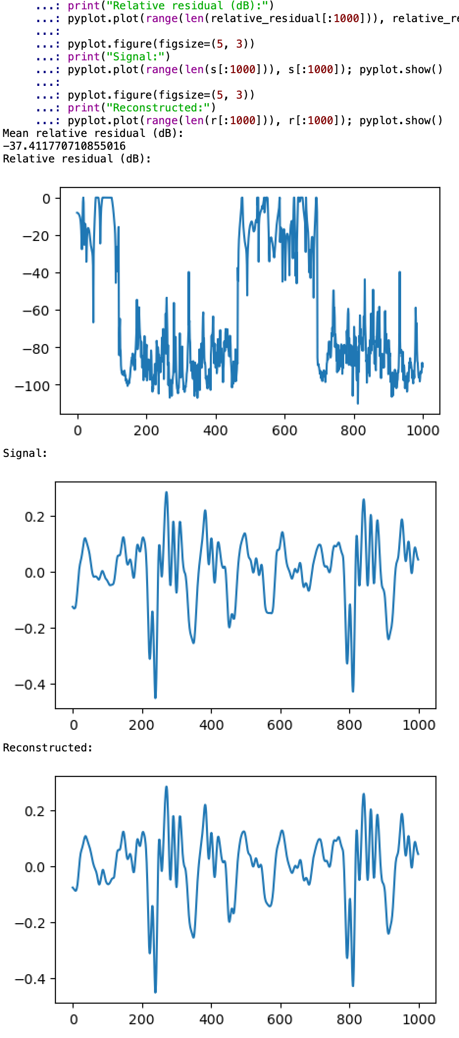
However, the voice pulses in analysis are already distorted. So then I already we can do the inverse resampling in the upsampling stage of WBVPM analysis to correct for non-stationary frequency, then it is redistorted according to the transformed fundamental frequency trajectory in the synthesis stage. This makes this method effectively invariant to modulations in fundamental frequency, so long as the modulation is less than the fundamental frequency and it is modeled well by the spline, which should be the case for modulation period is at least several voice pulses. PITCHED/UNPITCHED DECOMPOSITION - As mentioned in Bonada's thesis, WBVPM only models sinusoids, and thus residual in the input signal is encoded as flucuations between the spectra of voice pulses. I devised a post-processing technique to separate the voice pulses into sinusoidal and residual components. I have not actually implemented and test this yet, because as it is post-processing step, it will not improve the residual level, and in fact, will probably make it worse. The benefit of it is in the transformation stage, which is much harder to quantify and which I have not finished implementing. However, I believe this approach should work. The technique works as follows: a) First, for each voice pulse, and then for each harmonic of its spectra, we compute a spline based on the values of the amplitude of that harmonic in the voice pulse as well as a fixed number of surrounding voice pulses. b) Since the time delta between voice pulses can vary, we then resample each local harmonic spline with fixed steps in time. c) We compute the fourier transform of these resampled local harmonic trajectories d) We apply a low-pass and high-pass filter to separate it into low-frequency and high-frequency components. e) We then apply the inverse fourier transform to each of these. We can then sample the low pass trajectory at the time of the voice pulse to get the amplitude value of the denoised harmonic for that voice pulse. The same can be done for the high pass trajectory to obtain a pseudo-pulse representing the residual. These residual voice pulses can then be synthesized using the WBVPM synthesis method to obtain a time-domain residual signal which can be processed separately from the main harmonic signal. A significant source of error in this process presumably would come from the resampling step. This can be decreased by using a smaller time step, at an increased computational cost. However, the error could probably be greatly reduced by first calculating the difference between the original amplitudes and the amplitudes at the same times in a spline computed from the resampled harmonic spline before applying the band filters, this difference can later be added back to the low-pass amplitude trajectory. The denoised harmonic phase can also be computed via the same method, using Bonada's method for unwrapping phase across both frequency and time. The residual phase can be calculated by taking difference of the original phase from the denoised phase and dividing it by the residual amplitude. RESULTS: I have tested these improvements and obtained the following results for the aforementioned audio sample: Original WBVPM: -36.355dB Warp-correction improvement only: -36.74595dB Warp-correction & Resilient border interpolation in synthesis: -37.41177dB More research is needed to properly evaluate these improvements across more samples with more variety, and to see if these techniques still result in improvements with more accurate pitch and MFPA estimation and with proper handling of unvoiced/voiced frames.

Bump for visibility, merged with original thread.
I feel like I've been going insane over the last day. I've scoured every paper mention Excitation plus Resonance, but at least as far as I can tell, none of them actually mentioned the procedure for actually estimating the parameters of the EpR resonances. Even the expired patent for EpR doesn't seem to mention it. After thinking about it for a while, I attempted to come up with something. No idea if it will actually work though. The procedure I came up with is as follows: a) An amplitude spectrum representing N discrete sampled amplitudes of sinusoids in a frame or voice pulse is calculated such that for every index i in [0, N), Amp[i] is estimation of the value of the amplitude of a sinusoid having frequency i*F at a time or over a time period, where F is a constant frequency step. In the case of WBVPM, F is the fundamental frequency. b) A logarithmic amplitude spectrum comprising an array of N elements is created such that LogAmp[i] = log(Amp[i]) for i in [0, N), where N is the number of discrete values in the amplitude spectrum and Amp is the amplitude spectrum. c) A cubic natural spline LogInt comprising N - 1 segments is created from the values of the logarithmic amplitude spectrum and positions represent the frequency values of the sinusoids estimated in the amplitude spectrum. d) An array capable of holding up to 2N-2 objects representing the resonance parameters (frequency, amplitude, and bandwidth) is created and it's initial length is set to zero. e) For each segment S of the spline LogInt having index i and parameters offset o; span h; and coefficients a, b, c, and d (representing the cubic, quadratic, linear, and constant values, respectively); the following is performed: e) 1) The derivative of S is computed. e) 2) The roots of said derivative is computed, and for each of them, the following steps are performed: e) 2) a) It is checked whether the root, when the offset o and span h is accounted for, lies in the range [o, o+h] of segment S. If it does not, it is discarded and the further computation is skipped. e) 2) b) The value of the second derivative of the segment S is computed at the root. If it is not negative, the root is discarded and the further computation is skipped. e) 2) c) Then a resonance parameters object is appended to the end of the resonance parameters array, and that array's length is increased by one. The frequency value is set to the root. The amplitude value is set to the difference of the interpolated logarithmic amplitude spline value at the root and the value of the source curve at the root. The bandwidth value is set to the reciprocal of the negation of the second derivative of the segment at the root. f) An iterative refinement process of the resonances is performed for M iterations. For each iteration, the following is performed: f) 1) For each resonance O with index i in the resonance array, the following is performed: f) 1) a) A sum s is set to 0. f) 1) b) Then, for each resonance O2 (including resonance O) with index j in the resonance array, the sum is increased by the value of the resonance O2 at the frequency of the resonance O. f) 1) c) The difference between the sum s and the interpolated value of the logarithmic amplitude spline LogInt at the frequency of O is computed. It is multiplied by a fixed step size S and then the amplitude of O is subtracted by this value.
About three weeks ago, I promised that the following day, I would make a post the following day about a big update. I didn't say what it was about at the time, but it was going to be about the Excitation plus Resonance model. Unfortunately, I was not able to make the post at the time, and am sorry for that. However, I do have a significant update now. Back in April, I began to implement the Excitation plus Resonance model. The Excitation plus Resonance is model of the voice timbre spectrum. It consists of several parts actually, but the two main ones in terms of implementation difficult are the source curve and vocal tract resonances. The source curves approximates the frequency-domain response of the voice source, and the resonances correspond roughly to formants and are model using a modified version of the Klatt Formant. The problem lies not in implementing this model - it is actually very easy to do so - but rather estimating the parameters for this model, which is not given in any of the papers I've read. Back in April, I spent a couple days trying to create it. Ultimately, I came up with something that was quite poor quality, very slow, and required very specific parameters but accepted it. Much later though, I found that the exact method to estimate the source curve is actually given in the expired EpR patent. Not wanting to repeat my previous mistake, when I began to work on EpR, I searched extensively for the method used to estimate the resonances, but came up with nothing. Eventually, I began to trying figure it out myself. I started by recreating the data in the paper by annotating an image extracted from the paper in Photoshop and then running a python script on said annotated images. I would then compared the result of my approach on said recreated data to the paper's. I actually had been thinking about it long before my first attempt. I already had a method that I had conceived of. The main idea of this method was that the reciprocal of the second derivative could be used to approximate the bandwidths of the resonances. Initially, after having to make a few adaptions to the approach after realizing several things wouldn't work quite how I thought, the results vastly outperformed my initial expectations. There were several ideas that didn't work out, but overall I felt good at the end of the first day. I debated whether to continue trying or to just go with what I had. I decided that would go with what I had and make a post about it the following day, this about three weeks however. The next day however I decided to continue work instead. Initially, I was quite surprised that the second derivative reciprocal method even worked at all, so I overlooked many inadequacies. They were a lot larger than I had thought for some reason the previous. Specifically, in many of the most critical areas. It is worth noting that it is in a logarithmic scale (decibels), so apparently small errors in some areas can actually be very large. Furthermore, I discovered there was actually a mistake in the modified Klatt implementation, and that with the correct formulation, it performed much worse. Furthermore, the next day, I decided to recreate another sample from the paper, and it performed terribly. So I continued. I decided this time, I would not be satisfied until I had actually recreated it properly, no matter how long it took. Continued...
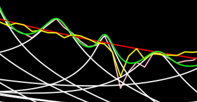
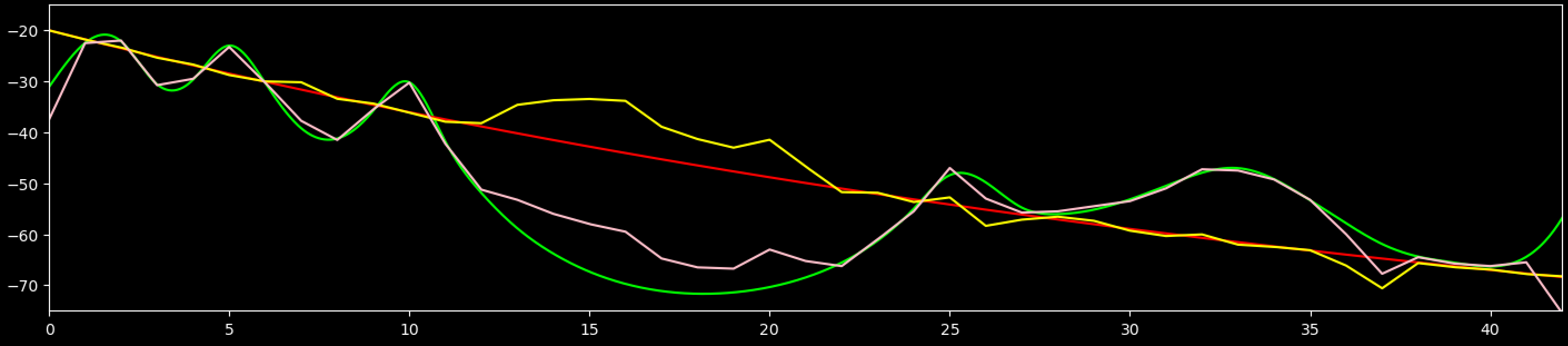
Three weeks later and 1,905 attempts later... Initially, I made quite some progress, however for over a week, I made basically no progress at all despite many hundreds of attempts. Finally, though, mainly in the past two to three days, I have made some major discoveries. Yesterday, I did a test that showed that combining an old idea I had ruled out with a new one showed significant progress. Just today, I have implemented that idea properly and made another significant improvement. While this new implementation is still flawed, and actually has major issues for the higher frequencies, I think it shows considerable potential. Besides, it is more simplified than the previous implementation and I have some clear ways forward. This new version solves many issues I had before and doesn't require many of contrived things I had to do before. One thing specifically it shows promise is in this section of the second recreated test sample. Here is that section from the paper: https://files.catbox.moe/ontyhu.png Here is the result from the old approach: https://files.catbox.moe/9uplbn.png And now here is the result from the new approach: https://files.catbox.moe/gzu3q8.png
1780199744985.png
- 98.46 KB
(2821x622)
I've got some good news, after three weeks and 2,279 attempts I've finally been able to recreate the EpR resonance estimator! I've written about a third of my post about it. I'm very tired though and have to go the bed. I will finish the post and post it tomorrow.
Also, can the title of the post be changed please since, as I said before, my idea at the time was wrong?
>>12555 Change the title to "Singing Voice Synthesizer project thread" and change the text of the first post to: """So I've been working on a project to create a singing voice synthesizer I'm basing it on the description in Jordi Bonada's PhD thesis "Voice Processing and Synthesis by Performance Sampling and Spectral Models". After a lot of trouble with getting TWM f0 estimation to work, I've finally gotten to implementing MFPA (Maximally Flat Phase Alignment". And amazingly, it seems to have worked first try."""
1000022408.jpg
- 254.37 KB
(600x600)

>>12557 Your wish has been granted.
I have finally finished writing the EpR post. I apologize for the delay. https://queuesevenm.wordpress.com/2026/06/02/recreating-the-excitation-plus-resonance-model/ TLDR: The bad news: I couldn't recreate the resonance estimation algorithm The good news: I created something even better.
Screen Shot 2026-06-25 at 12.11.32 AM.png
- 631.06 KB
(3346x1783)

I finally decided to start working on implementing an expression system.